Unidata Python Tutorial/Workshop

Helpful slides to learn about how to use Python for met data purposes.
https://unidata.github.io/unidata-python-workshop/events/fall2016.html

Python Basemap Background Image from ArcGIS MapServer

Click here for Jupyter Notebook

https://github.com/blaylockbk/pyBKB_v2/blob/master/demos/add_arcgis_image_to_basemap.ipynb
Python's Basemap toolkit has some default backgrounds you can load. To draw the background on your map you use m.bluemarble(), and m.shadedrelief(). These are really low resolution, so they aren't very useful if you zoom in on a specific area.

Alternatively, you can download higher resolution maps from the ArcGIS maps server. Here's how...
m.arcgisimage(service=maps, xpixels = 3500, dpi=500, verbose= True)

For the Salt Lake Valley, here's what each of the map backgrounds look like. You can plot anything on top of this :) 

 

To plot all of the availble maps I've made this script:
import matplotlib.pyplot as plt
import numpy as np
from functions_domains_models import *

from mpl_toolkits.basemap import Basemap


# Define the map boundaries lat/lon
domain = get_domain('salt_lake_valley')
top_right_lat = domain['top_right_lat']+.1
top_right_lon = domain['top_right_lon']-.1
bot_left_lat = domain['bot_left_lat']
bot_left_lon = domain['bot_left_lon']

## Map in cylindrical projection (data points may apear skewed)
m = Basemap(resolution='i',projection='cyl',\
    llcrnrlon=bot_left_lon,llcrnrlat=bot_left_lat,\
    urcrnrlon=top_right_lon,urcrnrlat=top_right_lat,)


map_list = [
'ESRI_Imagery_World_2D',    # 0
'ESRI_StreetMap_World_2D',  # 1
'NatGeo_World_Map',         # 2
'NGS_Topo_US_2D',           # 3
#'Ocean_Basemap',            # 4
'USA_Topo_Maps',            # 5
'World_Imagery',            # 6
'World_Physical_Map',       # 7     Still blurry
'World_Shaded_Relief',      # 8
'World_Street_Map',         # 9
'World_Terrain_Base',       # 10
'World_Topo_Map'            # 11
]

for maps in map_list: 
    plt.figure(figsize=[10,20])    
    ## Instead of using WRF terrain fields you can get a high resolution image from ESRI
    m.arcgisimage(service=maps, xpixels = 3500, dpi=500, verbose= True)
    m.drawstates()
    plt.title(maps)
    
    plt.savefig('00'+maps,bbox_inches="tight")

Python introduction for meteorologists

Some helpful slides from a python programming course for atmospheric science purposes:

https://sites.google.com/a/borealscicomp.com/zamg-scientific-python-aug-sep-2014/

Redefine Matplotlib defaults: Plotting Publication Quality Plots

The default python matplotlib settings don't look too good for publication quality work. So here I redefine some of matplotlib's default settings before I make a plot.

(see other parameters you can modify here: http://matplotlib.org/users/customizing.html)

import matplotlib as mpl

# Specify universal figure sizes acceptable for publication
# J.AtmosEnv
#        Figure width     |   Inches wide       
#   ----------------------+---------------------
#   1/2 page (1 column)   |  3.54 in. ( 90 mm)   
#   3/4 page (1.5 column) |  5.51 in. (140 mm)    
#   1   page (2 column)   |  7.48 in. (190 mm)    
#   ---------------------------------------------
# Image Resolution:  line graphs = 1000 dpi
#                    colorfilled = 500 dpi         
#                    web images  = 72 dpi             

label_font  = 10    
tick_font   = 8 
legend_font = 7

width=3.5
height=3

## Reset the defaults
mpl.rcParams['xtick.labelsize'] = tick_font
mpl.rcParams['ytick.labelsize'] = tick_font
mpl.rcParams['axes.labelsize'] = label_font
mpl.rcParams['legend.fontsize'] = legend_font

mpl.rcParams['figure.figsize'] = [width,height] 

mpl.rcParams['grid.linewidth'] = .25

mpl.rcParams['savefig.bbox'] = 'tight'
mpl.rcParams['savefig.dpi'] = 1000

Python multiprocessing plots

Often I need to create lots of plots. Wouldn't it be great if you could create all the plots at the same time rather than one by one. Summon the multiprocessing module! 

##---- Multiprocessing -------------------------------------------------------------------##

## There are a lot of data files for the two days of TDWR data that need to be plotted.

## We want to make these plots really fast, so use the multiprocessing module

## to create a separate plot on each available processor.

##      1) Place the plotting script in a function. 

##         The input (can only take one) is the file name of the data to be plotted

##      2) In the main program (bottom section of this script) 

##         a) creat a list of the file names (this simple loop is very fast)

##         b) count the number

##         c) creat the pool object p = multiprocessing.Pool(num_proc)

##         d) send each list item to the plot function with the pool function

## This method makes 475 plots in a few minutes rather than over an hour!!!

##---- Multiprocessing -------------------------------------------------------------------##

import multiprocessing #:)

import matplotlib.pyplot as plt

import numpy as np

#etc.

def make_plot(i):    

    # i is the name of the file we will open

    print i

    radar_time = i[8:23]

    

    DATETIME = datetime.datetime.strptime(radar_time,"%Y%m%d_%H%M%S")

    mesowest_time = DATETIME.strftime("%Y%m%d%H%M")

    

    string_time = DATETIME.strftime('%d %b %Y  %H:%M UTC')

    

    

    ### TDWR Radar Data (converted from .nids to .asc grid)

    text = 'SLC_TV0_'+radar_time+'.asc'

    this = np.flipud(np.genfromtxt(text,skip_header=6)) #flip the array

    # etc. plotting functions

## This is the good stuff...utilizing multiprocessors

if __name__ == '__main__':

    # List of file names we want to make plots for

    somelist = []

    for i in os.listdir('./'):

        if i[0:3]=='SLC' and i[-3:]=='asc': # get the file name of a TDWR file for all files

            somelist.append(i)      

    # Count number of processors

    num_proc = multiprocessing.cpu_count()

    p = multiprocessing.Pool(num_proc)

    p.map(make_plot,somelist)

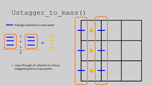
Python: WRF convert data on a staggered grid to mass point.

WRF output data has variables on a staggered grid (edges of grid boxes) and variables at a mass point (center of grid box). Sometimes it's necessary to convert the variables on a staggered grid to the mass points so you can plot U and V winds on the same latitude. Here are simple functions to convert the U and V variables on a staggered grid to the mass point grid.

https://github.com/blaylockbk/Ute_WRF/blob/master/functions/stagger_to_mass.py

Below is an explanation of how the function works...